library(BGLR)
library(asreml)
Loading required package: MatrixOnline License checked out Thu Mar 6 10:39:49 2025Loading ASReml-R version 4.2Mostly, I have been using the package asreml (The VSNi Team 2023) for fitting genomic prediction models. This year I started to read some papers about fitting GBLUP models. For example, I read the reaction norm paper (Jarquín et al. 2014) and the BGLR package paper (Pérez and Campos 2014). I noticed both papers used the BGLR package, so I wondered if I could get similar results with asreml. This post is an attempt to compare results from BGLR and asreml packages when fitting GBLUP models in single and multi-environment trials (MET).
To compare both packages, we are going to use a MET dataset from the BGLR package, which comprises 599 historical CIMMYT wheat lines. The phenotypic trait is the average grain yield of these 599 wheat lines, evaluated in four environments. The trait was standardized to have null mean and unit variance.
library(BGLR)
library(asreml)Loading required package: MatrixOnline License checked out Thu Mar 6 10:39:49 2025Loading ASReml-R version 4.2The first case is fitting a GBLUP for a single environment (here we consider the first).
data(wheat, package = "BGLR")
# ?wheat  # to know more about it

# phenotypes
wheat.Y <- as.data.frame(wheat.Y)
colnames(wheat.Y) <- paste0("y", 1:4)
rownames(wheat.Y) <- NULL
wheat.Y$name <- as.factor(1:nrow(wheat.Y))  # fake genotype names
y <- wheat.Y[, 1]  # get yield from first environment
head(wheat.Y)
y1 y2 y3 y4 name
1 1.6716295 -1.72746986 -1.89028479 0.0509159 1
2 -0.2527028 0.40952243 0.30938553 -1.7387588 2
3 0.3418151 -0.64862633 -0.79955921 -1.0535691 3
4 0.7854395 0.09394919 0.57046773 0.5517574 4
5 0.9983176 -0.28248062 1.61868192 -0.1142848 5
6 2.3360969 0.62647587 0.07353311 0.7195856 6The columns y1 to y4 represent the yield of each environment. I used fake numbers (1 to 599) to name each genotype in the column name.
# markers
X <- wheat.X
n <- nrow(X)
p <- ncol(X)
dim(X)
[1] 599 1279We have 599 individuals and 1279 markers.
We are going to evaluate the CV1 scheme (predicting unobserved genotypes), therefore 100 random genotypes will be hold as testing set. Remember, we are using the phenotypes from the first environment stored in y. In the BGLR package, we can mask the test set by setting the phenotypes to NA:
yNA <- y
set.seed(123)
tst <- sample(1:n, size = 100, replace = F)
yNA[tst] <- NA
The tst object holds integers that shows which rows are to be used as the testing set, and we are going to use them to calculate the test set accuracy.
I am computing the genomic relationship matrix as described in the BGLR paper (Pérez and Campos 2014, see Box 9):
X <- scale(X, center = T, scale = T)
G <- (X %*% t(X)) / p  # same as tcrossprod(X) / p
rownames(G) <- colnames(G) <- levels(wheat.Y$name)
dim(G)
[1] 599 599G[1:5, 1:5] 1 2 3 4 5
1 1.11819432 0.06109962 0.05387119 0.2473040 0.44643151
2 0.06109962 1.44217931 1.42698671 0.1103435 -0.01189792
3 0.05387119 1.42698671 1.44527589 0.1062722 -0.00525292
4 0.24730400 0.11034351 0.10627223 0.8733090 0.22284413
5 0.44643151 -0.01189792 -0.00525292 0.2228441 0.84811023Fitting GBLUP in BGLR requires us to set a linear predictor (ETA).
In this case, we are using only one kernel, i.e., the covariance matrix G. If you want to check the iterations, set verbose = T.
ETA <- list(list(K = G, model = "RKHS"))
fm1 <- BGLR(y = yNA, ETA = ETA, nIter = 5000, burnIn = 1000,
            saveAt = "GBLUP_", verbose = F)
pred_gblup_bglr <- data.frame(
  name = wheat.Y[tst, "name"],
  y = y[tst],
  yhat = fm1$yHat[tst]
)
cor(pred_gblup_bglr$y, pred_gblup_bglr$yhat)  # correlation between observed and predicted values
[1] 0.5601514Note: if you get a LAPACK error in Ubuntu, for example, try changing the defaults of BLAS and LAPACK 1.
Fitting GBLUP in asreml requires us to pass the covariance matrix G in the vm object. Now, we can just fit the model removing the testing samples with wheat.Y[-tst, ].
mod1 <- asreml(y1 ~ 1, random = ~ vm(name, source = G, singG = "PSD"),
               data = wheat.Y[-tst, ])
ASReml Version 4.2 06/03/2025 10:39:55
LogLik Sigma2 DF wall
1 -232.3355 0.8552212 498 10:39:56
2 -224.1149 0.7898886 498 10:39:56
3 -214.8656 0.6987314 498 10:39:56
4 -209.2359 0.6131716 498 10:39:56
5 -207.4308 0.5509318 498 10:39:56
6 -207.3177 0.5335289 498 10:39:56
7 -207.3163 0.5315242 498 10:39:56pred_gblup_asreml <- data.frame(
y = wheat.Y[tst, "y1"],
predict(mod1, classify = "name")$pvals[tst, c("name", "predicted.value")]
)ASReml Version 4.2 06/03/2025 10:39:56
LogLik Sigma2 DF wall
1 -207.3163 0.5313973 498 10:39:56
2 -207.3163 0.5313950 498 10:39:56
3 -207.3163 0.5313899 498 10:39:56cor(pred_gblup_asreml$y, pred_gblup_asreml$predicted.value)[1] 0.5596302Comparing both packages:
comp1 <- data.frame(
  package = c("BGLR", "asreml"),
  varG = c(fm1$ETA[[1]]$varU, summary(mod1)$varcomp[1, "component"]),
  varE = c(fm1$varE, summary(mod1)$varcomp[2, "component"]),
  accuracy = c(cor(pred_gblup_bglr$y, pred_gblup_bglr$yhat),
               cor(pred_gblup_asreml$y, pred_gblup_asreml$predicted.value)))
comp1
package varG varE accuracy
1 BGLR 0.5859860 0.5388088 0.5601514
2 asreml 0.5736408 0.5315242 0.5596302where varG is the genetic variance, varE is the residual variance, and accuracy is the Pearson’s correlation between observed and predicted values (considering only the test set). The results are similar.
pred <- merge(pred_gblup_bglr, pred_gblup_asreml, by = "name")
plot(pred$yhat, pred$predicted.value,
     xlab = "BGLR predictions", ylab = "asreml predictions")
abline(coef = c(0, 1), col = "blue", lty = 2)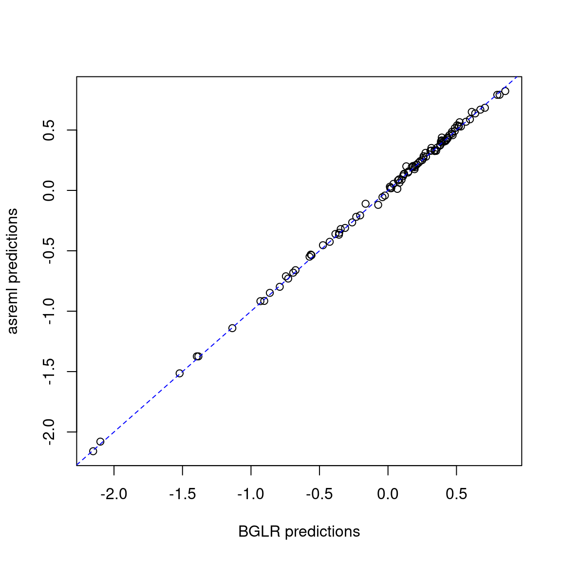
Now let’s consider when we have more than one environment. This data has four.
We reshape the data from wide (four environments, one column per environment) to long (one column for all environments stacked).
wheat.Y.long <- reshape(wheat.Y, direction = "long", varying = 1:4,
                        timevar = "env", sep = "")
wheat.Y.long$id <- NULL
rownames(wheat.Y.long) <- NULL
wheat.Y.long$env <- as.factor(wheat.Y.long$env)
dim(wheat.Y.long)
[1] 2396 3head(wheat.Y.long) name env y
1 1 1 1.6716295
2 2 1 -0.2527028
3 3 1 0.3418151
4 4 1 0.7854395
5 5 1 0.9983176
6 6 1 2.3360969tail(wheat.Y.long) name env y
2391 594 4 1.7915575
2392 595 4 1.6596565
2393 596 4 0.5543848
2394 597 4 1.8487169
2395 598 4 2.6928141
2396 599 4 0.3813174Remember, name are the genotypes, and env are the environments.
Now we mask again, but now the response is in the long format. We will search for the rows where the genotypes were in the test set in the previous example.
ylong <- wheat.Y.long[, "y"]
ylongNA <- ylong
set.seed(123)
tstlong <- as.integer(
  rownames(wheat.Y.long[wheat.Y.long$name %in% wheat.Y[tst, "name"], ])
)
ylongNA[tstlong] <- NA
length(tstlong)
[1] 400As the genotypes are repeated across environments, we need to expand the covariance matrix G to account for the repetitions. To do this, we perform \(Z G Z'\), where \(Z\) is the incidence matrix (also called design matrix) that connects genotypes to phenotypes, \(G\) is the genetic relationship matrix, and \(Z'\) is the incidence matrix transposed, as explained in Jarquín et al. (2014).
Z <- as.matrix(model.matrix(lm(y ~ name - 1, data = wheat.Y.long)))
ZGZt <- Z %*% G %*% t(Z)
dim(ZGZt)
[1] 2396 2396Note that the \(Z G Z^{'}\) matrix has dimension \(n \times n\), i.e., it matches the dimension of repeated genotypes across environments. You can play with Z to see how it looks like.
Now we pass the kernel \(Z G Z'\) (instead of \(G\)) in the linear predictor.
ETA <- list(list(K = ZGZt, model = "RKHS"))
fm2 <- BGLR(y = ylongNA, ETA = ETA, nIter = 5000, burnIn = 1000,
            saveAt = "MET_BGLUP_", verbose = F)
pred_gblup_bglr <- data.frame(
  name = wheat.Y.long[tstlong, "name"],
  env = wheat.Y.long[tstlong, "env"],
  y = ylong[tstlong],
  yhat = fm2$yHat[tstlong]
)
cor(pred_gblup_bglr$y, pred_gblup_bglr$yhat)
[1] 0.3111166In asreml we can pass directly the \(G\) matrix without expanding it.
mod2 <- asreml(y ~ 1, random = ~ vm(name, source = G, singG = "PSD"),
               data = wheat.Y.long[-tstlong, ])
ASReml Version 4.2 06/03/2025 10:40:39
LogLik Sigma2 DF wall
1 -902.1607 0.8549988 1995 10:40:39
2 -899.6476 0.8455182 1995 10:40:39
3 -897.4152 0.8330925 1995 10:40:39
4 -896.5900 0.8236879 1995 10:40:39
5 -896.4757 0.8190706 1995 10:40:40
6 -896.4751 0.8187290 1995 10:40:40p <- predict(mod2, classify = "name")$pvals[, c("name", "predicted.value")]ASReml Version 4.2 06/03/2025 10:40:40
LogLik Sigma2 DF wall
1 -896.4751 0.8187204 1995 10:40:40
2 -896.4751 0.8187203 1995 10:40:40
3 -896.4751 0.8187202 1995 10:40:40pred_gblup_asreml <- data.frame(
name = wheat.Y.long[tstlong, "name"],
env = wheat.Y.long[tstlong, "env"],
y = wheat.Y.long[tstlong, "y"]
)
pred_gblup_asreml <- merge(pred_gblup_asreml, p, by = "name")
cor(pred_gblup_asreml$y, pred_gblup_asreml$predicted.value)[1] 0.311257Comparing both packages:
comp2 <- data.frame(
  package = c("BGLR", "asreml"),
  varG = c(fm2$ETA[[1]]$varU, summary(mod2)$varcomp[1, "component"]),
  varE = c(fm2$varE, summary(mod2)$varcomp[2, "component"]),
  accuracy = c(cor(pred_gblup_bglr$y, pred_gblup_bglr$yhat),
               cor(pred_gblup_asreml$y, pred_gblup_asreml$predicted.value)))
comp2
package varG varE accuracy
1 BGLR 0.1736191 0.8177197 0.3111166
2 asreml 0.1691422 0.8187290 0.3112570The results are similar.
pred_met <- merge(pred_gblup_bglr, pred_gblup_asreml, by = c("name", "env"))
plot(pred_met$yhat, pred_met$predicted.value,
     xlab = "BGLR predictions", ylab = "asreml predictions")
abline(coef = c(0, 1), col = "blue", lty = 2)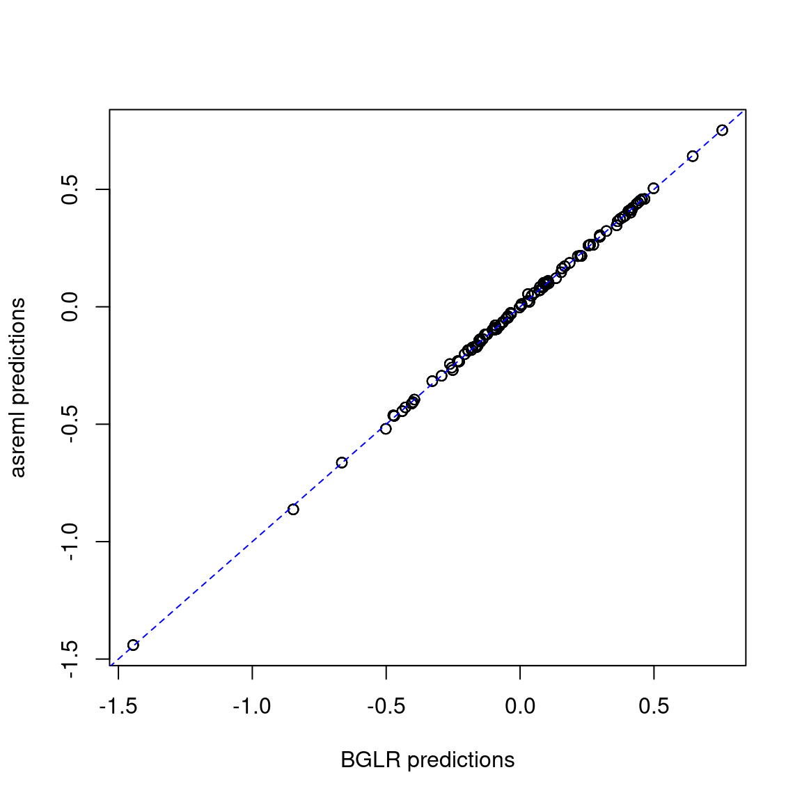
In both cases (single model and MET model), the varG differed a little bit among packages. I don’t know why is that, but if you know I would be happy to see the explanation. Apart from that, the results are very similar.
I hope you enjoyed this comparison! Let me know if you have any comments or issues.
sessionInfo()R version 4.4.1 (2024-06-14)
Platform: x86_64-apple-darwin20
Running under: macOS Sonoma 14.6.1
Matrix products: default
BLAS: /Library/Frameworks/R.framework/Versions/4.4-x86_64/Resources/lib/libRblas.0.dylib
LAPACK: /Library/Frameworks/R.framework/Versions/4.4-x86_64/Resources/lib/libRlapack.dylib; LAPACK version 3.12.0
locale:
[1] en_US.UTF-8/en_US.UTF-8/en_US.UTF-8/C/en_US.UTF-8/en_US.UTF-8
time zone: America/Chicago
tzcode source: internal
attached base packages:
[1] stats graphics grDevices utils datasets methods base
other attached packages:
[1] asreml_4.2.0.355 Matrix_1.7-2 BGLR_1.1.3
loaded via a namespace (and not attached):
[1] vctrs_0.6.5 cli_3.6.4 knitr_1.49 rlang_1.1.5
[5] xfun_0.50 generics_0.1.3 jsonlite_1.8.9 data.table_1.16.4
[9] glue_1.8.0 colorspace_2.1-1 htmltools_0.5.8.1 scales_1.3.0
[13] rmarkdown_2.29 grid_4.4.1 tibble_3.2.1 munsell_0.5.1
[17] evaluate_1.0.3 MASS_7.3-64 fastmap_1.2.0 yaml_2.3.10
[21] lifecycle_1.0.4 compiler_4.4.1 dplyr_1.1.4 pkgconfig_2.0.3
[25] htmlwidgets_1.6.4 rstudioapi_0.17.1 truncnorm_1.0-9 lattice_0.22-6
[29] digest_0.6.37 R6_2.6.0 tidyselect_1.2.1 pillar_1.10.1
[33] magrittr_2.0.3 tools_4.4.1 gtable_0.3.6 ggplot2_3.5.1 See section “Selecting the default BLAS/LAPACK” of the tutorial Improving R Perfomance by installing optimized BLAS/LAPACK libraries↩︎